Documentation
Introduction
The Single Cell Database (scDB) integrates single-cell transcriptome data from 32 research projects registered in the Korea BioData Station (K-BDS), covering both human and mouse samples. Analysis results are provided at two levels: Study-level (SCS) offers comprehensive analyses integrating all samples within a project, while Data-level (SCD) provides detailed analyses for individual library runs. For data generated using 10x Genomics sequencing platforms, we apply standardized pipelines beginning from raw FASTQ data, including preprocessing, quality control, clustering, cell type annotation, differential expression analysis, cell-cell interaction analysis, and functional enrichment analysis. Detailed descriptions of each pipeline and the methodologies employed are available below.
Analysis Pipeline (v2025.12)
| Name | Type | Version |
|---|---|---|
| Reference genome | File |
Homo sapiens (GRCh38,p14) Mus musculus (GRCm39) |
| Cell Ranger | Software | 8.0.1 |
| Python | Software | 3.10.11 |
| pandas | Package | 2.3.1 |
| numpy | Package | 1.26.4 |
| scanpy | Package | 1.9.4 |
| anndata | Package | 0.10.9 |
| openai | Package | 1.100.0 |
| R | Software | 4.3.1 |
| Seurat | Package | 5.3.0 |
| valiDrops | Package | 0.1.0 |
| topGO | Package | 2.52.0 |
| CellChat | Package | 2.2.0 |
Study-level Analysis
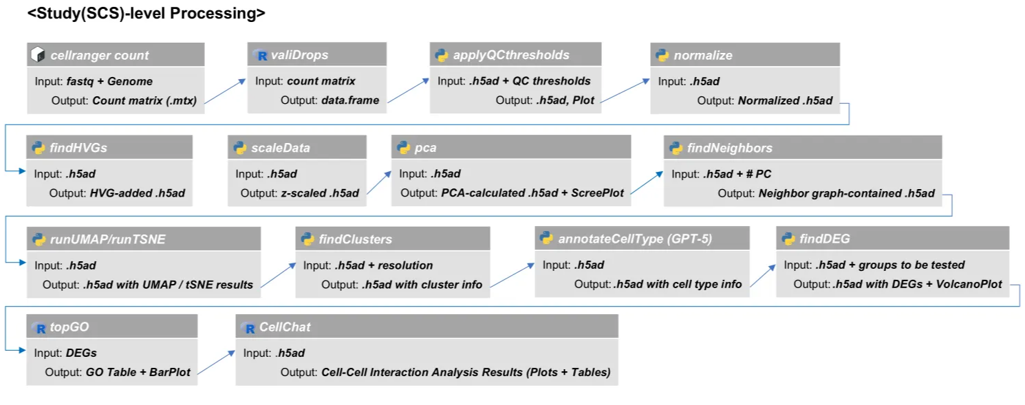
Step 1. Convert FASTQ to count matrix
# Bash
cellranger count \
--id=sample_ID \
--sample=sample_prefix \
--fastqs=/path/to/fastq_data \
--transcriptome=/path/to/reference \
--localcores=6 --localmem=24 \
--nosecondary
Step 2. Data preprocessing
•Remove empty droplets
# R
library(DropletUtils)
library(valiDrops)
library(scuttle)

# 1. Read Raw 10X Count Matrix into SingleCellExperiment (SCE) object
sce <- read10xCounts("/path/to/raw_feature_bc_matrix")
rownames(sce) <- scuttle::uniquifyFeatureNames(rowData(sce)$ID, rowData(sce)$Symbol) # Set feature names (genes) to be unique for compatibility

# 2. Run valiDrops for Empty Droplet Filtering
valid <- valiDrops(counts(sce), label_dead = TRUE)

# 3. Subset SCE Object to Keep Only Valid Cells
sce_filtered <- sce[, colnames(sce) %in% valid$barcode]
sce_filtered@colData <- cbind(sce_filtered@colData, valid[, 2:ncol(valid)]) # Attach the valiDrops metadata to the filtered SCE object

# 4. Save Filtered Count Matrix
write10xCounts(
    x = sce_filtered@assays@data$counts,
    barcodes = colnames(sce_filtered),
    gene.id = rowData(sce_filtered)$ID,
    gene.symbol = rowData(sce_filtered)$Symbol,
    gene.type = rowData(sce_filtered)$Type,
    version = "3",
    path = "/path/to/filtered_feature_bc_matrix"
)
•Data QC and filtering
# Python
# 1. Load Filtered 10X Count Matrix
adata = sc.read_10x_mtx(
    path='/path/to/filtered_feature_bc_matrix',
    var_names='gene_symbols', gex_only=True
)

# 2. Calculate QC metrics (Number of genes, UMI count, Mitochondrial gene percentage)
adata.var['mito'] = adata.var_names.str.startswith(('MT-', 'mt-'))
sc.pp.calculate_qc_metrics(adata, qc_vars=["mito"], inplace=True)

# 3. Cell Filtering
adata = adata[adata.obs['log1p_total_counts'] > 0, :]
adata = adata[adata.obs['log1p_n_genes_by_counts'] > 0, :]
adata = adata[adata.obs['pct_counts_mito'] < 100, :]

# 4. Save File
adata.write("/path/to/adata_qc_passed_concat.h5ad")
Step 3. Data preprocessing
# Python
# 1. Normalization
sc.pp.normalize_total(adata, target_sum=1e4) # Normalize each cell to 10,000 UMI
sc.pp.log1p(adata) # Log transform (log(x+1))

# 2. Highly Variable Gene (HVG) Selection
sc.pp.highly_variable_genes(
    adata,
    flavor='seurat',
    min_mean=0.0125,
    max_mean=3,
    min_disp=0.5,
    inplace=True
)

# 3. Scaling (Standardize data)
sc.pp.scale(
    adata,
    zero_center=True,
    max_value=None
)
Step 4. Dimension reduction and clustering
# Python
# 1. Principal Component Analysis (PCA)
sc.pp.pca(
    adata,
    n_comps=50,
    zero_center=True,
    svd_solver='auto',
    random_state=0
)

# 2. Neighbor Graph Generation (Calculate cell-to-cell similarity based on PCA results)
sc.pp.neighbors(
    adata,
    n_neighbors=15,
    n_pcs=None,
    use_rep=None,
    knn=True,
    method='umap',
    metric='euclidean',
    random_state=0
)

# 3. Non-linear Dimensionality Reduction (tSNE, UMAP)
sc.tl.tsne(
    adata,
    n_pcs=None,
    use_rep=None,.
    perplexity=30,
    early_exaggeration=12,
    learning_rate=1000,
    random_state=0
)

sc.tl.umap(
    adata,
    min_dist=0.5,
    spread=1.0,
    n_components=2,
    init_pos='random',
    random_state=0
)

# 4. Clustering - Using the Leiden algorithm
sc.tl.leiden(
    adata,
    resolution=1.0,
    use_weights=True,
    random_state=0,
    directed=None,
    n_iterations=-1
)
Step 5. Automated cell type annotation
This step leverages the GPT-5 model to automatically annotate cell types based on marker genes, tissue, and organism information. The prompt in annotateCelltype_GPT5.py is sent to the OpenAI API, which requires a valid API key. This step produces adata_cellType_annotated.h5ad file as a result.
annotateCelltype_GPT5.py
# Bash
python annotateCelltype_GPT5.py \
    --input-dir /path/to/analysis/input/ \
    --output-dir /path/to/analysis/output/ \
    --groupby leiden \
    --groups all \
    --log2fc-abs-thr 0.25 \
    --sample-info-file /path/to/sample_info.csv
Step 6. Differential gene expression analysis
# Python
# 1. Identify Cluster Marker Genes
sc.tl.rank_genes_groups(
    adata,
    groupby='leiden',
    groups='all',
    method='t-test',
    corr_method='benjamini-hochberg',
    tie_correct=False
)
Step 7. Functional analysis
•GO analysis
# R
library(topGO)
library(org.Hs.eg.db)

# 1. Select Upregulated DEGs for a Specific Cluster (i)
allmarkers = read.csv('/path/to/DEG_results')
targetGenes = subset(
    allmarkers,
    allmarkers$logfoldchanges > 0.5 & allmarkers$pvals_adj < 0.05
)$names

# 2. Create the Gene Universe Vector (0: Background, 1: Target Gene)
backgroundGenes = allmarkers$names
allGene = factor(as.integer(backgroundGenes %in% targetGenes))
names(allGene) = backgroundGenes

# 3. Create the topGOdata object
tgd = new(
    "topGOdata",
    ontology = "BP",
    allGenes = allGene,
    nodeSize = 10,
    annot = annFUN.org,
    mapping = "org.Hs.eg.db", # Use "org.Mm.eg.db" for mouse
    ID = "symbol"
)

# 4. Run GO Enrichment Test
resultTopGO.elim = runTest(
    tgd,
    algorithm = "elim",
    statistic = "Fisher"
)

# 5. Extract and Filter the Result Table
topGOResults = GenTable(
    tgd,
    Fisher.elim = resultTopGO.elim,
    orderBy = "Fisher.classic",
    topNodes = 200,
    numChar = 1000L
)
topGOResults = topGOResults[topGOResults$Fisher.elim < 0.05, ] # Final P-value cutoff
•Cell-cell interaction analysis
# Python
# 1. Convert Adata to SingleCellExperiment Object
adata = sc.read_h5ad('/path/to/h5ad')
r_command = 'ad = as(adata_prev, "SingleCellExperiment"); saveRDS(ad, "/path/to/adata_to_sce.rds")'
with localconverter(anndata2ri.converter):
    rpy2.robjects.globalenv['adata_prev'] = adata
    rpy2.robjects.r(r_command)
# R
# 2. Load SCE Object
sce <- readRDS(paste0(INPUT_PATH, "/", args[["--prefix"]], "/path/to/adata_to_sce.rds"))
sce@assays@data$logcounts <- sce@assays@data$X
sce@assays@data$X <- NULL

# 3. Create CellChat object and Set Database
cellchat <- createCellChat(sce, group.by = "celltype")
cellchat@DB <- get("CellChatDB.human") # Use "CellChatDB.mouse" for mouse

# 4. Run Preprocessing Steps
cellchat <- cellchat %>%
    subsetData() %>%
    identifyOverExpressedGenes(
        do.fast = TRUE,
        group.by = "celltype",
        min.cells = 10) %>%
    identifyOverExpressedInteractions() %>%
    smoothData(
        adj = get("PPI.human"), # Use "PPI.mouse" for mouse
        alpha = 0.5)

# 5. Compute Communication Probability and Infer Pathways
cellchat <- cellchat %>%
    computeCommunProb(
        raw.use = FALSE,
        type = "triMean") %>%
    filterCommunication(
        min.cells = 10,
        rare.keep = TRUE) %>%
    computeCommunProbPathway(thresh = 0.05) %>%
    aggregateNet(thresh = 0.05)
Data-level Analysis
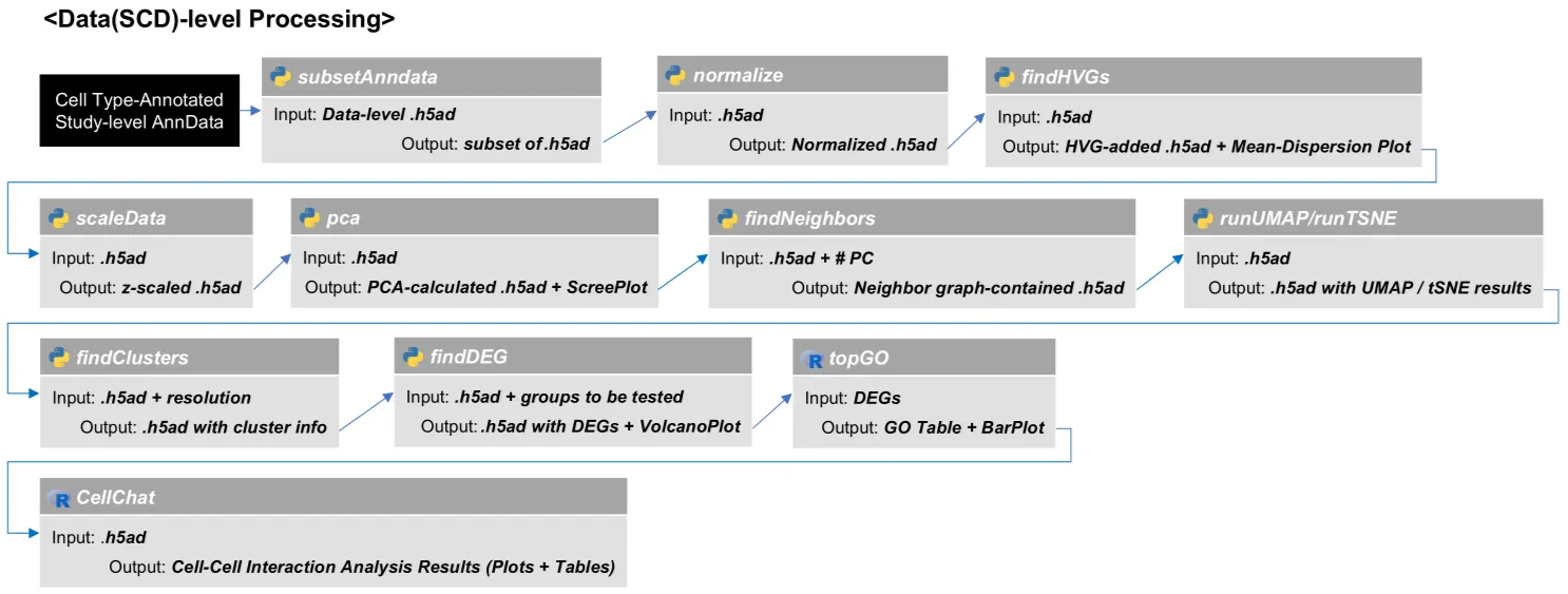
Step 1. Subset data-level anndata
# Python
# 1. Load the Fully Processed Study-level AnnData (with cell type annotation)
adata = sc.read_h5ad("/path/to/adata_cellType_annotated.h5ad")

# 2. Load Study-level Preprocessed AnnData
adata_raw = sc.read_h5ad("/path/to/adata_qc_passed_concat.h5ad")

# 3. Apply the Final Metadata from the Processed Object
adata_raw.obs = adata.obs.copy()

# 4. Subset Preprocessed AnnData to a specific Data ID (e.g., 'SCD20000010')
adata_subset = adata_raw[["Data_Acession_ID"]]]
Step 2. Normalization and scaling
# Python
# 1. Normalization
sc.pp.normalize_total(adata, target_sum=1e4) # Normalize each cell to 10,000 UMI
sc.pp.log1p(adata) # Log transform (log(x+1))

# 2. Highly Variable Gene (HVG) Selection
sc.pp.highly_variable_genes(
    adata,
    flavor='seurat',
    min_mean=0.0125,
    max_mean=3,
    min_disp=0.5,
    inplace=True
)

# 3. Scaling (Standardize data)
sc.pp.scale(
    adata,
    zero_center=True,
    max_value=None
)
Step 3. Dimension reduction and clustering
# Python
# 1. Principal Component Analysis (PCA)
sc.pp.pca(
    adata,
    n_comps=50,
    zero_center=True,
    svd_solver='auto',
    random_state=0
)

# 2. Neighbor Graph Generation (Calculate cell-to-cell similarity based on PCA results)
sc.pp.neighbors(
    adata,
    n_neighbors=15,
    n_pcs=None,
    use_rep=None,
    knn=True,
    method='umap',
    metric='euclidean',
    random_state=0
)

# 3. Non-linear Dimensionality Reduction (tSNE, UMAP)
sc.tl.tsne(
    adata,
    n_pcs=None,
    use_rep=None,.
    perplexity=30,
    early_exaggeration=12,
    learning_rate=1000,
    random_state=0
)

sc.tl.umap(
    adata,
    min_dist=0.5,
    spread=1.0,
    n_components=2,
    init_pos='random',
    random_state=0
)

# 4. Clustering - Using the Leiden algorithm
sc.tl.leiden(
    adata,
    resolution=1.0,
    use_weights=True,
    random_state=0,
    directed=None,
    n_iterations=-1
)
Step 4. Differential gene expression analysis
# Python
# 1. Identify Cluster Marker Genes
sc.tl.rank_genes_groups(
    adata,
    groupby='leiden',
    groups='all',
    method='t-test',
    corr_method='benjamini-hochberg',
    tie_correct=False
)
Step 5. Functional analysis
•GO analysis
# R
library(topGO)
library(org.Hs.eg.db)

# 1. Select Upregulated DEGs for a Specific Cluster (i)
allmarkers = read.csv('/path/to/DEG_results')
targetGenes = subset(
    allmarkers,
    allmarkers$logfoldchanges > 0.5 & allmarkers$pvals_adj < 0.05
)$names

# 2. Create the Gene Universe Vector (0: Background, 1: Target Gene)
backgroundGenes = allmarkers$names
allGene = factor(as.integer(backgroundGenes %in% targetGenes))
names(allGene) = backgroundGenes

# 3. Create the topGOdata object
tgd = new(
    "topGOdata",
    ontology = "BP",
    allGenes = allGene,
    nodeSize = 10,
    annot = annFUN.org,
    mapping = "org.Hs.eg.db", # Use "org.Mm.eg.db" for mouse
    ID = "symbol"
)

# 4. Run GO Enrichment Test
resultTopGO.elim = runTest(
    tgd,
    algorithm = "elim",
    statistic = "Fisher"
)

# 5. Extract and Filter the Result Table
topGOResults = GenTable(
    tgd,
    Fisher.elim = resultTopGO.elim,
    orderBy = "Fisher.classic",
    topNodes = 200,
    numChar = 1000L
)
topGOResults = topGOResults[topGOResults$Fisher.elim < 0.05, ] # Final P-value cutoff
•Cell-cell interaction analysis
# Python
# 1. Convert Adata to SingleCellExperiment Object
adata = sc.read_h5ad('/path/to/h5ad')
r_command = 'ad = as(adata_prev, "SingleCellExperiment"); saveRDS(ad, "/path/to/adata_to_sce.rds")'
with localconverter(anndata2ri.converter):
    rpy2.robjects.globalenv['adata_prev'] = adata
    rpy2.robjects.r(r_command)
# R
# 2. Load SCE Object
sce <- readRDS(paste0(INPUT_PATH, "/", args[["--prefix"]], "/path/to/adata_to_sce.rds"))
sce@assays@data$logcounts <- sce@assays@data$X
sce@assays@data$X <- NULL

# 3. Create CellChat object and Set Database
cellchat <- createCellChat(sce, group.by = "celltype")
cellchat@DB <- get("CellChatDB.human") # Use "CellChatDB.mouse" for mouse

# 4. Run Preprocessing Steps
cellchat <- cellchat %>%
    subsetData() %>%
    identifyOverExpressedGenes(
        do.fast = TRUE,
        group.by = "celltype",
        min.cells = 10) %>%
    identifyOverExpressedInteractions() %>%
    smoothData(
        adj = get("PPI.human"), # Use "PPI.mouse" for mouse
        alpha = 0.5)

# 5. Compute Communication Probability and Infer Pathways
cellchat <- cellchat %>%
    computeCommunProb(
        raw.use = FALSE,
        type = "triMean") %>%
    filterCommunication(
        min.cells = 10,
        rare.keep = TRUE) %>%
    computeCommunProbPathway(thresh = 0.05) %>%
    aggregateNet(thresh = 0.05)